Mathematical Beauty Series: The Binomial Theorem

Welcome to the inaugural entry of the newest series on this blog: The Mathematical Beauty Series.

While many posts on this blog have been taking highlight of various topics in mathematics that I take time to appreciate, I don’t think I’ve done a post that really takes a deep dive on a specific topic akin to my retrospectives on my personal blog (The Hiro’s Blog, for reference). With that being said, I’d like to now introduce a series that does so and really marvel at topics that encapsulate this abstract concept known as “Mathematical Beauty”, something I previously hinted at in my post on the Pythagorean Theorem. To start, let’s start with The Binomial Theorem, something I first encountered as a sophomore in Algebra II.

To start, we should look at how the Binomial Theorem is defined. This was something I did not have done for me in that Algebra II class, rather it was in my Combinatorics course in college:

Seems like a lot to dissect there, eh? What on earth is that giant Greek letter doing there? Why are there giant parentheses there with two numbers that seem to have a missing fraction bar? How can high schoolers even begin to understand that this was what they are seeing? We will need to examine different topics before connecting them together to form understanding of what that formula is even saying.

Part 1: Combinatorics

To start, we need to talk Combinatorics, an area of Mathematics primarily concerned with counting. The Whole Numbers are usually the only numbers that are delved into within this area (0, 1, 2, 3…). Example topics include Graph Theory, Venn Diagrams, and even Probability.

One of the most well-known topics, however, regards Permutations and Combinations. I pose two questions.

1. A 100 yard dash track event has eight people participating. How many ways can the podium look?
2. The board of trustees is looking to add three people for its inaugural incarnation. 8 people are in the running. How many distinct groups of people could form the board of trustees?

The key to both of these questions is the idea of “how many”, and the idea is that we have to effectively count “how many”. Additionally, there is an implication that no “object” (in both problems, the “objects” are individual people) can be selected twice, i.e. no repetition. There is, however, a subtle difference between the two questions. The first question has an implied order, while the second does not, and this plays to the difference between permutations (which is the subject of the first question) and combinations (which is the subject of the second question).

Let us look at the first one. As I previously stated, there is an implied order with this question, given the problem statement, “How many ways can the podium look?” The insinuation here is that we will have a 1st place/Gold, 2nd place/Silver, and 3rd place/Bronze. With eight people competing to be on the podium, there are eight possible choices for who can finish first. Once that is done, only seven are left for second place, then six for third place. We then multiply these numbers (8, 7, and 6) to determine how many ways the podium can look: 8 x 7 x 6 = 336.

Because of the implied order, examples like this one are examples of ones involving Permutations, where members of a set of things (numbers, people, logos, etc.) are arranged in a sequence or linear order. As mentioned before, this differs from Combinations, where there is no sense of a sequence or linear order.

Let us now look at the second question. Notice how the numbers are the same: given we have 8 people running for the three positions on the board, we have to figure out how many unique configurations we can make. Using our earlier understanding, we have 8 spots for the first position, 7 spots for the second, 6 spots for the third. The main difference now is that the positions are indistinguishable, meaning we must account for any times we count the same combination more than once. To do this, we must consider how many positions there actually are. Because we have three, we must consider how many ways that the three positions (not the people!) can be arranged if there was an order: 3 x 2 x 1 = 6. Thus, once we account for the 336 potential permutations, we must divide this number by 6 to account for over-counts, which results in 56.

So notice how when there is an order, we will have more possibilities. When there is no order, we have less because we discard permutations that are regarded as the same combination (ex. “ABC” is regarded as the same combination as “CBA” as they both contain “A”, “B”, and “C”). In order to generalize the situations, we should first approach one important concept: factorial.

You’ve probably seen some jokes like these on the internet:

As it turns out, this is a tongue-in-cheek joke about how the factorial works: n! is defined as the product of the first n natural numbers. Thus, 5! = 1 x 2 x 3 x 4 x 5 = 120, which is the result of the exercise in the joke. The factorial of a number is very important for combinations, as they are necessary to determine the number of permutations and combinations.

On the first problem involving the podium, notice how we had 8 x 7 x 6, which is part of 8!. However, 5 x 4 x 3 x 2 x 1, which is 5! (funny coincidence!), is missing. We can then restate that what we were doing was 8! divided by 5!. How we can relate 8 and 5 is that 5 is equal to 8 – 3, and notice how 3 is the number of people that we were trying to “permute”. So in general, given any n objects to be permuted into k slots, we have P(n, k) = n!/(n-k)!. In terms of finding combinations, recall how we were also dividing further by k!, so we have the following…

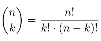
The “object” (pun kind of intended) on the left side of the equation has a specific name that we will discuss later, but it is most often read as “n choose k” and is sometimes written (most often in high school and on Texas Instruments graphing calculators) as “_nC_k” or “_nC_r” (by consequence, P(n, k) is sometimes written as “_nP_k” or “_nP_r“). For example, in the second problem, we were effectively computing “8 choose 3”, which is equal to 56.

In the event that k is somehow bigger than n, _nC_k is said to be 0. However, most often k is less than or equal to n. Regardless, n and k are whole numbers, meaning that 0 can be a value for both. That then begs the question of what it means to “choose 0” or what on earth “0 choose 0” means. For the former, choosing zero “objects” means to choose nothing, and that it is only possible to do so 1 way. That then means that there is only one way to choose nothing out of nothing, which is what the implication of “0 choose 0” is. This also implies that if we have ₀C₀, by using the formula, we will have to consider what 0! is equal to. However, given what we have come to the conclusion of how when we choose nothing, we are choosing “0”, and in that event, we have n! divided by the product of n! and 0!. If this is to be 1, then 0! must also be equal to 1. This is a more conceptual way of defining what 0! is, and there are other ways that force us to set the value of 0! to 1 so that the mathematics makes sense.

Anyhow, I encourage you all to do your own little mini examples of generating “n choose k”, perhaps by saying “here are some distinct letters, how many ways can you choose ‘k’ of them”. For example, with A, B, and C, there is 1 way to choose none, 3 ways to choose one (A, B, and C), 3 ways to choose 2 (A and B, A and C, and B and C), and 1 way to choose all three. List these out somewhere, because there will be a strange coincidence…

Part 2: Pascal’s Triangle

The next part is going to be interesting, as we will talk about Pascal’s Triangle, named after French mathematician Blaise Pascal, having noted of the arrangement’s “eccentricities” and useful applications in his own document that was published posthumously (Treatise on Arithmetical Triangle, or Traité du triangle arithmétique). However, it was studied around the world prior to his time, and it is known as Yang Hui’s Triangle in China after the mathematician. His predecessor Jia Xian was the first to discover the triangle in China, but Jia’s original book was lost and it was Yang who was the first to publish the findings (and named Jia as a source).

Now, let us discuss how to even generate it. First, at the top of the triangle is a 1, which forms the “0 row”. The actual “first” row is made of two 1s. Then, along the outermost edges of the triangle are all 1s, but generating the interior requires using the above numbers by finding their sum. Thus, in the second row, the middle number is 1 + 1, or 2. Then, in the third row, we have two numbers in the middle, but we have a 1 and a 2 above each slot, thus we find that their sum, 3, goes in each one. This next animation should illustrate it:

Hey… don’t these numbers look familiar? Notice how those numbers that I asked you to list are the one and the same! Each “nth” row gives the values of “n choose k” from k = 0 to k = n. Let us look at the next several rows…

As you can see, the numbers can get quite big! Notice how our earlier computed value of “8 choose 3”, or 56, shows up in its proper slot. Neato!

So we’ve already built a connection between combinations and this eerie triangle. There is one more thing we need to examine…

Part 3: Binomial Expansions

This next section is more algebra-heavy, so fair warning.

Let us discuss binomials. A binomial is an algebraic expression that is a subset of polynomials, which in turn are algebraic expressions composed of variables, exponents made of whole numbers, coefficients, constants, along with addition, subtraction, or multiplication as additional operations. A monomial is a polynomial made of just one term, while binomials are polynomials that is the sum of two monomials. An implication is that due to there being two terms, the individual monomials are NOT like-terms, meaning that the operation separating the two is either addition or subtraction, hence why a binomial is the “sum” (or difference if at least one of the terms has a negative coefficient, although such a distinction is largely negligible).

For example, the most common binomial that students study is either “a + b” or “x + y” (and their counterparts “a – b” or “x – y”), specifically their square. For simplicity, we will look at the former (a + b) and consider when they are raised to a whole number power.

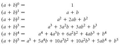
To start, let us consider (a + b)⁰. Given that any number (aside from 0) raised to the 0 power is equal to 1, that means that (a + b)⁰ = 1 (again, as long as a + b does not equal 0).

Then, let us go to (a + b)¹. Raising to the first power has no restrictions, and it represents another rather trivial case as it evaluates to the base. Thus, (a + b)¹ = a + b. Keep in mind that our coefficients for both variables are 1 right now.

Next, we examine (a + b)². Most often, folks will make the mistake of saying, “Oh! It’s just ‘a² + b²‘!” When in reality, that is most often not the case. There are occasions where it is, but such occasions are not only rare, but also quite uninteresting. When we really have to multiply both quantities, you must consider EVERY part. (a + b)² = (a + b) x (a + b), which in turn, is equal to a x (a + b) + b x (a + b). Visually, this is what we are doing:

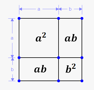
Thus, what we actually have is (a + b)² = a² + 2ab + b². As you can see, if (a + b)² were to simply be a² + b², then 2ab = 0, meaning one of a or b is 0, making such a computation absurdly trivial.

Again, (a + b)² = a² + 2ab + b². Note how the coefficients here are 1, 2, and 1. Sense a pattern?

Now let’s look at (a + b)³. Again, you can simply “split” this expression into (a + b)¹ x (a + b)², and we know what both expressions are equal to: a + b and a² + 2ab + b², respectively. Thus, we must evaluate (a + b) x (a² + 2ab + b²). You can do this for yourself to confirm that we will arrive at a³ + 3a²b + 3ab² + b³. The coefficients are 1, 3, 3, and 1.

…huh?

Anyway, let’s go further to (a + b)⁴. When we repeat the process from before, we will arrive at a⁴ + 4a³b + 6a²b² + 4ab³ + b⁴. The coefficients are 1, 4, 6, 4, and 1. Wait a minute…

Part 4: Connecting Parts 1, 2, and 3

It keeps getting crazier.

Look at how all these coefficients are lining up so eerily. 1, then 1 and 1, then 1, 2, 1, then 1, 3, 3, 1… doesn’t such an arrangement look familiar? Again, you can keep going on and on but it seems like we can’t escape the triangle. And recall how the numbers in the triangle are really just the numbers that result from determining “n choose k”.

For example, in (a + b)⁴, the coefficient of the a⁴ term is 1, or “4 choose 0”. Then for the a³b term, we have 4 as the coefficient, or “4 choose 1”, and so forth. Perhaps we can really refine what we are seeing and generalize it. At the a⁴ term, there is also a hidden b⁰ term, which we know to be equal to 1 (if b were 0 we wouldn’t really be talking about this stuff now, would we :p), and the values of n and k are 4 and 0, respectively. Thus, at every term, we are really looking at a^n-kb^k which has a coefficient of “n choose k”.

There now remains how we can truncate everything given that we are summing similar terms. This is where we have to introduce sigma notation.

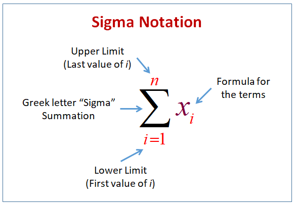
The image above gives a good idea of a generalization of how summation with sigma notation works. If there are a group of terms with similar characteristics that we wish to sum, sigma notation is used to group them into a sort of “shorthand”. Below the upper case sigma is the indication of what the index is (i) and the lower bound of the index, with the upper limit of the index being atop the sigma. The indices from the lower bound to the upper bound are to rise by an increment by 1 for any summation written in sigma notation. This all might seem very complex (it definitely is for anybody learning it for the first time, including myself back in the day), so it’s best to look at an example to get a better understanding:

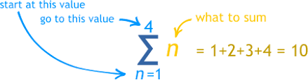
In the above example, if we wanted to put “1 + 2 + 3 + 4” into sigma notation, we’d look at how many terms there are (4), decide on both a lower and upper bound for the index. Since the lowest and highest terms of our sum are “1” and “4”, it is best to start at 1 and end at 4. The terms we are summing are effectively the indices from 1 to 4, meaning all we need to write to the right of the upper case sigma is the index (in this case, we choose “n”).

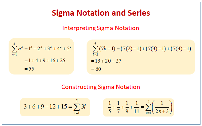
I believe it is important to start with very basic examples of sigma notation in order to properly understand what’s really going on, and only then should one proceed with the blog. Above are some very basic examples for you to analyze, and I suggest you look online for some others before trying to come up with examples of your own. For those who already understand it, however, let us proceed.

In our example with the binomial expansions (example: (a + b)³ = a³ + 3a²b + 3ab² + b³), we saw a progressive pattern with what the terms were going to be. Each coefficient to each term was related to “n choose k”, while the exponents on the terms were changing (as the ones on “a” decreased by 1, the ones on “b” increased by 1). Using our earlier generalization, we had “a^n-kb^k has a coefficient of ‘n choose k'”, we can use this to our advantage when coming up with constructing the generalization in sigma notation. Because we are considering the general case of (a + b)ⁿ, we know that the upper bound of our summation should be “n”. For the lower bound, though, we should examine what our initial term is. In every case, we have just aⁿ, and when looking at how this translates to the general case, k must be equal 0. Thus, we set 0 as the lower bound, and this also allows us to choose “k” as the index. Thus, we have the following…

Part 5: The Binomial Theorem and Mathematical Beauty

This is the end result of our findings: The Binomial Theorem in full.

The fact that we can connect seemingly unrelated concepts in counting problems, a peculiar triangular arrangement of numbers, and a specific topic in algebra is a perfect example of “Mathematical Beauty.” This idea of “Mathematical Beauty” rears its head in many different ways and is often whimsical and can catch even the greatest of mathematicians off-guard. Think of the discoveries of concepts that have Mathematical Beauty akin to a “EUREKA!” moment where things all of a sudden come together with a sudden, giant rush.

So if you thought that this was crazy, wait until I post more in these series.